CS 7638 - AI For Robotics

🔍 Overview

AI for Robotics provides an introduction to various navigation and localization methods in uncertain environments. The content covers traditional methods more-so than machine learning approaches. This involves implementing various location estimation, path finding, and controls methods from scratch. The projects are all done in Python, and involve implementing methods, which typically run over some simulated environment.

Much of the content covers the basics of Thrun's textbook, Probabilistic Robotics. Most of the following figures will be from this.

*I took this course Summer 2019, contents may have changed since then

🏢 Structure

• Six assignments - 28% (of the final grade)
• 3 Projects- 45%
• Mini Project - 7%
• Final Project - 20%

Assignments

These assignments (problem sets) are the same as those on the Udacity course, and are relatively straightforward. I believe they are just meant to reinforce concepts to prepare for projects

1. Probability and Localization - Basic probability, Bayes Rule, and location estimation
2. Kalman Filters - Gaussian distributions, Kalman filters, and matrix operations
3. Movement and Sensing -Car-like robot kinematics, object sensing, and localization
4. Path finding - Admissible heuristics and motion
5. Smoothing - Cyclic paths and smoothing
6. SLAM - Online simultaneous localization and mapping

Projects

There are three main projects, and mini project, and a final project, all of which are due throughout the semester. They all involved submitting code and passing test cases. I will describe the three projects, followed by the mini project, and then the final project.

• Asteroids - Navigate through an "asteroid field" to a goal by steering and estimating future asteroid locations
• Mars Glider - Use a particle filter to localize a glider based on a known map and noisy sensor measurements
• Ice Rover - Implement a SLAM module and robot controls to navigate through a world
• Rocket PID (Mini) - Find optimal controls parameters to control the output of engines on a simulated rocket
• Warehouse (Final) - Guide a robot to retrieve and deliver packages in a continuous warehouse environment

📁 Probability and localization

Topics are not centered around completing assignments, but rather the projects, so I will try to introduce the relevant topics and then discuss the projects in more depth.

A robot's understanding of an environment through navigations and interactions can be summarized by the above diagram.

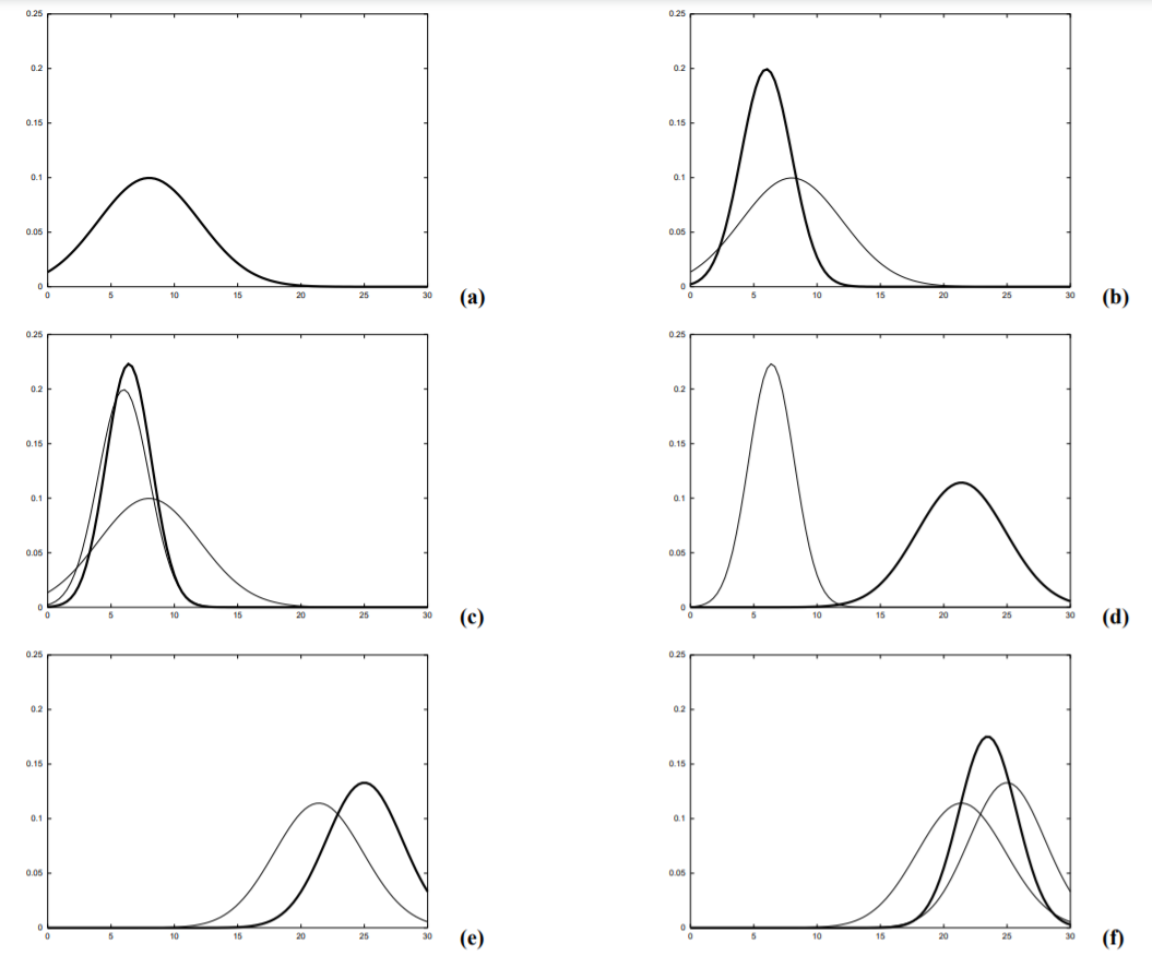
As a simple example, let's take a robot in a 2D plane that can sense a door, and move. It has a map of the area and tries to localize its position.

At the above initial position, before sensing or moving, it has no idea where it is. On the y axis, bel(x) represents the belief of its position, the probability that is at location x. It is uniform across all locations.

Now, it uses its sensor. p(z|x) is the conditional probability z given x, which is simply the chance that we sense a door given the position x. Each door is equally likely, and when we are at the center of the door, there is a higher probability. The rest of the areas still have a low chance, as our sensor could be faulty- we don't want to completely rule them out. The bel(x) is now equal to exactly p(z|x), as we previously had no knowledge on our location.

This time, our robot moves. It has not sensed again yet. Notice that the peaks of each have shifted but are reduced. This is because our movement estimation is not perfect, so each time we move, the confidence in location decreases a bit.

The robot senses a door again. The probability of a sense occurring given location x, the p(z|x), remains the same. However, compared to the first time with no knowledge, we had an estimate of already being at the second door, so this time, we are fairly confident that we are there, as shown in the updated bel(x). Due to the potential of a faulty sensing, we don't want to discount the other possibilities of locations.

The final action we take is moving. Like what happened before, our certainty was reduced again, but because we were previously so confident , we still have a confident estimate in our location.

Consider how these distributions would look if our sensor was less accurate vs perfect?

These update rules can be mathematically represented by Bayes Theorem. With these variables, that would be:

$p(x|z) = \frac{p(z|x)\ bel(x)}{p(z)}$

Each time we sense a door, the posterior distribution, $p(x|z)$, the which is the probability of location X given the sense outcome Z, is updated through the likelihood, $p(z|x)$, which was discussed already, with the prior, $bel(x)$, which was our previous estimate of where we were. This is normalized by $p(z) \equiv \int p(z|x)bel(x)dx$, which is derived from total probability. For the next iteration the new prior is equal to the previous posterior. This process of estimation is known as a Bayes Filter.

📁 Kalman Filters

This is the most common implementation of the Bayes Filter.

There are ample resources out there for the specifics of Kalman Filters, so I'll just share two visuals I like.

The following visualizes the change in belief when there is motion and sensing.

I shared the following visualization in my Computer Vision review, which shows an estimate of location based on noisy measurements. It is tracking my mouse (my screen capture omitted my mouse though, sorry). Try out the demo here.

💻Project 1 - Asteroids

We apply the concepts before to navigate through a 2D asteroid field.

There are two main tasks- to estimate the locations of the asteroids using a Kalman Filter, and to navigate away from obstacles and reach the goal in a timely manner.

Results

We first implemented the Kalman Filter from scratch. This was tested on a variety of test cases, so we had to get the hyperparameters tuned to this problem to pass them.

For navigation, we are able to turn left and right, as well as decelerate and accelerate.

Below is one of the tests for navigation.

The little black cursor is our ship.

Its belief of the asteroids is the colored dots. When the estimate is too far off, the color changes to red, but the ship acts based on the estimated dot. Close call at the end!

There were many approaches students used that could pass the test cases, we didn't need to get too complex. Mine involved a fitness function which prioritized moving forward and deducted from being close to asteroids. I would predict the locations of the ship and asteroids for the next frame on each action, and choose best outcome based on the fitness function.

📁 Particle Filters

Particle Filters are often used for object localization, both for tracking, as well as for SLAM (simultaneous localization and mapping). It is essentially a clever sample-efficient search technique which estimates the likelihood of a state across many locations, reassigns weights, and resamples according to those most likely.

💻Project 2 - Mars Glider

Our task is to localize a glider which is currently descending Mars. We have a map of the terrain height of the area it will land in, but do not know its exact location. There is only a height sensor, and we need to utilize a particle filter to estimate the glider's location.

Results

A particle filter is an efficient way to locate the glider as it efficiently breaks down the search problem. At the start, we have no idea where we are, so we want to check as many points on the map as possible. We understand the movement of the glider, so we can sweep through the terrain and resample to the most likely areas.

In the first gif below, we initialized with many particles, which are represented by the black markers. There are many possible candidates at the beginning, as we have not had enough readings to hone in on the exact location. The purple dot represents our estimate, which is an average of all the particle locations. The red marker (hard to see) is the true location of the glider.

The second gif is after many iterations- the number of particles is reduced because we are confident of our location and can be more computationally efficient.

The challenge for this problem is that the sensor can be very noisy, so a vanilla implementation of a particle filter won't succeed. One technique used is fuzzing, which selects some of the particles to randomly change their direction and position. This helps maintain a more robust tracker.

Fun fact. Cruise missiles navigate by a similar technique, called Terrain Contour Matching, to localize. GPS is not nearly fast or accurate enough to achieve the precision needed.

📁 PID Control

A proportional-integral-derivitive (PID) controllers use a feedback loop to calculate and control process variables to reach a stable target result. Applications include an industrial machine, or even steering a car to follow a desired path.

Proportional refers to the bias, the difference between the current result and the expected result. A P-controller would usually fail to converge to target value and oscillate around it instead.

Derivative keeps track of the error over time. A PD-controller can see that the change in error has improved, so the output can be dampened accordingly. This can prevent the steady state error and enable the system to converge to the target value.

However, there may be an error in your actual output variable, for example misaligned wheels, which may require you to turn slightly right to actually steer straight. This is the systemic bias. Below, the system is offset from the target (the axis line) and converges at the dotted line.

The Integral notes the total bias up to a certain point, so if improvement isn't seen, the output can be adjusted further.

All together, these three are added with non-negative coefficients $K_p, K_d, K_i$

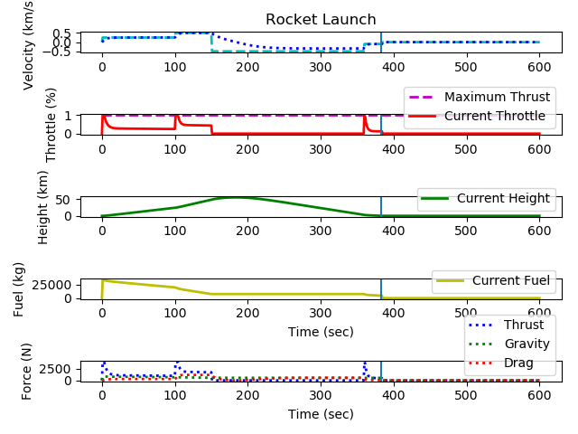
💻Mini Project - Rocket PID

We have a simulated rocket launch and landing and are given target velocities to reach. This assignment involved tuning the $K$ variables to control the output thrust. There are some constraints, like fuel and throttle capacity.

📁 SLAM

Simultaneous Localization And Mapping (SLAM) involves creating a map of an unknown environment while keeping track of your location. The Roomba is the SLAM robot we all know and love.

You can immediately see its importance for autonomous vehicles, UAVs, and planetary rovers.

There are many techniques for this, and this course goes over Graph SLAM, which localizes an agent and nearby landmarks from noisy motion estimates and sensor measurements.

These two posts cover more detail about the specific implementation from the lectures:

https://garimanishad.medium.com/everything-you-need-to-know-about-graph-slam-7f6f567f1a31

https://medium.com/@krunalkshirsagar/graph-slam-a-noobs-guide-to-simultaneous-localization-and-mapping-aaff4ee91dee

💻Project 3 - Ice Rover

A robot has arrived in an unknown location on an ice sheet. There are a set of beacons that are scattered randomly, and do not move. We can measure the distance between the robot and each nearby beacon, but do not know their coordinates.

A set of sample sites is provided, as well as their true coordinates. These can be measured in the same way as the beacons. Our goal is to navigate to each site and "collect" a sample, which requires being near the site within a certain distance.

Results

We implement the matrix operations for Graph SLAM to solve this.

The graded tests involved varied number of beacons, sample sites, measurement noise, and motion noise. Unfortunately, there aren't any visuals I can provide here.

📁 Path Finding and Smoothing

A* is a graph traversal and path search algorithm, and achieves better performance by using heuristics.

A common heuristic is using the Euclidean distance to the goal, which is the straight line distance between two points. A* will decide the next node to visit based on the cost to get there, and the heuristic. If we use an admissible heuristic, we are guaranteed to find an optimal solution. An admissible heuristic is one that never overestimates the cost to the goal.

In a continuous environment, we can improve upon this by smoothing our output paths.

We can achieve this path by optimizing for the two following equations:

$minimize: (x_{smooth,\ i}-x_i)^2$

$minimize: \alpha(x_{smooth, i} - x_{smooth, i - 1})^2$

For the first equation, we are trying to minimize the difference between the originally calculated path and the calculated path. For the second equation, we try to minimize the difference between two adjacent points on the smoothed path. Parameter $\alpha$ weights the importance of smoothing, where higher values result in a smoother but further deviated path.

If we were to only optimize for the first, the path would remain unchanged. If only the second, then the path would be the shortest distance: a straight line to the destination.

💻Final Project - Warehouse

Our robot navigates through a warehouse to retrieve and deliver multiple packages. This involves using A* to create an optimal plan of navigation. The first part of the project is in a discrete environment, and the second one is continuous, so path smoothing is needed.

There's not much else to it other than implementing these details and adjusting hyperparameters accordingly. In the above, we (blue dot) need to retrieve each package (red square), and drop them off in the green area.

⏩ Next Steps

The general theme of the course is high-level concepts related with self-driving cars, though there is not too much depth for each topic. We begin to piece together the technical system involved, which involves making sense of many noisy inputs to ultimately form an accurate assessment and action choice. A natural next step would be to learn more about the system-level design, or look into more complex approaches for topics like SLAM.