CS 6476 - Computer Vision

🔍 Overview

Computer vision is the broad term of being able to understand and manipulate image or video using mathematical and machine learning methods.

This course provides an introduction to computer vision, from theory to practice. The large focus is on traditional imaging methods- filtering, transforms, tracking. This involves writing some algorithms from scratch, but mostly utilizing existing implementations, largely in OpenCV, and tuning them to complete a certain task.

While the class does not focus on state-of-the-art research, it provides the backbone to begin to understand it. The final project provides a good opportunity to put that to action, which is a more open-ended assignment where you can use modern deep learning methods.

*I took this course Spring 2019, contents may have changed since then

🏢 Structure

• Six assignments - 70% (of the final grade)
• Final project - 15%
• Final exam - 15%

Assignments

For each of these assignments, you are provided a code skeleton, unit tests, and image assets. The amount of code to implement varies, but typically there is a file of empty functions which have unit tests (local as well as remote autograded). There is an experiment file which requires small modifications to generate output images for your report.

1. Images as Functions - Basic functions over image arrays, mostly to practice numpy and OpenCV
2. Detecting Traffic Signs and Lights - Utilizing hough transforms and color masking for robust multiple sign detection and labelling
3. Introduction to Augmented Reality - Pinpointing markers through template matching and corner detection, and projecting images onto the plane through
4. Motion Detection - Flow algorithms to detect motion and interpolate images
5. Object Tracking and Pedestrian Detection - Kalman filter and particle filter for tracking moving objects under occlusions and changing appearences
6. Image Classification - Facial detection and recognition

Final Project

You select one of four final topics. Each consists of a coding portion as well as a 5 page written report, which discusses your process, results, and comparison to state-of-the-art methods. You are not restricted to a specific approach for the most part, so students end up using various methods for their submissions

1. Classification and Detection with Convolutional Neural Networks - Digit recognition system which returns a sequence of digits from a real-world image. Trained on the Street View House Number dataset
2. Enhanced Augmented Reality - Improving robustness from assignment 3, Introduction to AR, by inserting a plane into a scene without markers
3. Stereo Correspondence - Finding depth variation for objects in a scene using stereo correspondence algorithms and disparity maps
4. Activity Classification using Motion History Images - Classify activities such as walking, clapping, or boxing through Hu moments to characterize MHIs.

I chose the Classification with CNNs project, so I will talk about that one in further detail

📖 Assignment 1 - Images as Functions

This assignment covers basic matrix operations and image operators, such as splicing, color filtering, and adding noise. The lectures for all modules are viewable on Udacity.

An image is represented as a matrix, where each element represents a pixel's RGB value, as well as depth and transparency if applicable. For example, the following matrix is an image of horizontal, solid colors. These RGB values are mixed to represent every color that we can interpret.

[[255, 0, 0], [255, 0, 0], [255, 0, 0] ... ], # Blue
[ ...                                      ],
[[0, 255, 0], [0, 255, 0], [0, 255, 0] ... ], # Green
[ ...                                      ],
[[0, 0, 255], [0, 0, 255], [0, 0, 255] ... ], # Red
[ ...                                      ]

Really, the purpose is to start to get your feet wet and familiarize yourself with numpy. This assignment is a good gauge for whether or not you are prepared for the course.

Results

Here are some of the outputs generated for the assignment's report

Top left: the original image I selected.

Top right: green and blue channels swapped, causing the green peppers to change hue.

Bottom left: The difference between the image with itself shifted by two two pixels. This is a basic edge detector, with some tweaks we have the Sobel operator, which is more robust.

Bottom right: Gaussian noise is added to the green channel.

📖 Assignment 2 - Detecting Traffic Signs and Lights

Line detection has many applications in computer vision, perhaps most notably for determining road lanes. For this assignment, line detection is applied to simulated and real-world street sign classification.

The Hough Transform can be used for efficient line detection, and it is conceptually rather simple. There are three main steps for this method:

• Calculate edge features (Sobel operator or another filter)
• Map each point for the edges onto a parameterized plane and accumulate counts
• Find the highest counts and map back to the original plane

Above are the graphs for the mapping step. Each point on the line (left graph) is associated with the curve of the same color on the parameterized plane (right graph), and they all intersect at the point which defines the line in the edge-detected image.

The mapping can be adjusted for detecting circles too, as well as any shape.

Results

OpenCV already has an implementation of the Hough transform, which we utilize for line detection and then extend those results to locate and classify signs. The basic pseudocode is as follows:

def find_stop_sign(image):
  image = denoise(image)
  edges = find_edges(image)
  lines = find_lines(edges) # Utilize cv2.HoughTransform
  potential_stop_sign = []
  for line in lines:
    # Is there a set of lines that geometrically form a stop sign?
    add_to_potential_stop_sign(potential_stop_sign) 

This second output above was more challenging, involving noise as well as many more signs which increase the number of output lines for each detection, resulting in a harder search problem. For example, if you simply fed in every detected line in the image (around 30), and you try to classify a stop sign which has 8 edges, there are 30 choose 8 combinations of lines, which is around 6 million. How might you reduce that space for efficient detection?

Here's a real world example of detecting the no entry sign. I applied the same algorithm and parameters to this image as for the previous problems.

📖 Assignment 3 - Introduction to Augmented Reality

We look at two major components in augmented reality: determining the location to project images on, and how to actually display that graphic with respect to the environment.

Template matching in computer vision is finding the location of a provided template within an image. We can take the difference between every pixel in a patch and the template, for each patch in the image, to output a likelihood of the template existing at each location

We can see in the above image the result of this operation with a template as their face. Every pixel in the left image is the difference between the template and the patch, centered around that pixel. There is a distinct bright point at the location of the face.

This operation would be very inefficient for many objects and scales, and there are many faster and robust techniques, especially for face detection, which will be discussed in assignment 6.

Homography (or perspective transform, projective transform) in computer vision describes the transformation between two planes in an image. This is necessary in augmented reality as projecting an image onto an image will usually require a shift in perspective.

The math is actually not too complex, and only involves basic linear algebra, and we do have to calculate the homography matrix from scratch for the assignment. The details, further applications, and examples are well described in this OpenCV tutorial.

Results

The first part of the assignment involves simple template matching in a simulated environment. Here, we just want to detect exact copies of the template, which is the circular marker

For the final output of the assignment, we project an image of our choice into a noisy and shifting scene.

The high-level steps are as follows:

for frame in video:
  frame = denoise(frame)
  markers = find_markers(frame)
  # Find the matrix for transforming the template image to the marker locations
  homography = find_homography(my_image, markers)
  image = project_image_to_frame(frame, my_image, homography)

📖 Assignment 4 - Motion Detection

Content

Motion detection for objects in a scene has vast applications from people analysis, camera motion estimation, object location estimation, and even frame interpolation.

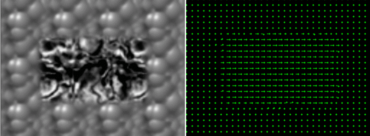
The Lucas-Kanade method (LK) is used for optical flow estimation. At a high level, it solves for the flow vector between two consecutive images in the X and Y directions.

The above is a moment from the middle of a video which ran LK and overlaid the flow vectors. LK flow estimation assumes small displacements, and it can be applied in a hierarchical manner to detect larger changes.

We can utilize the detected flow vectors for frame interpolation. For example, say the displacement of an object is 5 pixels, which was detected from Lucas Kanade. We can utilize this flow to reverse the pixels in the direction of the flow by half to generate an estimate of the object positioned in between the provided locations.

Results

The first output on the right shows the flow vectors detected between the two images in the left gif. Note that a flow is estimated for every single pixel, but the output is sampled for visualization purposes.

In the gif below, we are provided three images, the car door closed, opened, and halfway opened. My result was not the smoothest output.

In contrast to object motion detection in the images before, the following gif shows the flow vectors laid over a static scene but moving camera. You can see that the movement estimation is accurate in the areas with many features, like in the center. However, in locations like the top left corner where nearby pixels have similar colors, the flow estimation is much more noisy.

📖 Assignment 5 - Object Tracking and Detection

Kalman filters takes a series of noisy measurements over time, and produces accurate estimates based on the prior estimate, current measurement, and dynamics model. They are used widely, and while simple, result in almost magically reliable results for many applications like GPS.

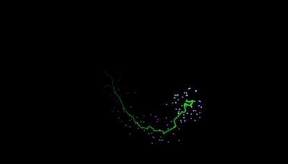
One of my favorite Kalman Filter demonstrations is from this website (gif below). It estimates mouse position based on noisy measurements that are generated from your mouse as dots. On the site, you can adjust the dynamics, noise, and other variables.

Particle Filters are often used for object localization, both for tracking, as well as for SLAM (simultaneous localization and mapping). It is essentially a clever sample-efficient search technique which estimates the likelihood of a state across many locations, reassigns weights, and resamples according to those most likely.

Results

Given a template image to track, we utilize particle filters to estimate the location. For each frame, the particles, as shown below, calculate the likelihood that the template is centered at that location. Then, the existing particles are randomly relocated according to the likelihood weights, with more being assigned to the higher weighted particles. The movement can be tracked by the dynamics model, which in this case, is simply gaussian noise applied each iteration to the particles.

Tracking becomes more complex when the object changes in appearance. We can dynamically change the template by talking a combination of the existing template by the best predicted particle in the current frame, as is shown below.

In the following output, we face further challenges, where the target changes in both appearance and size, and is also temporarily occluded by oncoming individuals. When the woman is blocked, you can see in my implementation that the particles stop movement until the target reemerges.

📖 Assignment 6 - Image Classification

The Viola-Jones object algorithm is an efficient and robust face detection framework.

This method is driven by Haar-like features, as shown below. When applied to an image, the light regions are subtracted by the dark regions. Over the faces, we can expect the lighter regions to be of higher light intensity on the face than the dark section (cheeks are lighter than the nose in the first image, eyes are darker than cheeks in the second). The sums over these areas can be computed very quickly in O(1) time by utilizing integral images.

The haar-like features are generated from training images, and classifiers are trained most commonly by Adaboost. Each feature is used as its own classifier, and the chain is how it runs so fast. Although a sliding window with different scales are used, most are quickly rejected by the first classifier, so the computation is efficient.

Results

Unfortunately there isn't much to show for this assignment, except this one blurry detected face used for the output, as is shown here. I promise we used Viola-Jones, and didn't just draw a blue rectangle!

💻 Final Project - Classification and Detections with CNNs

The Street View Housing Numbers dataset consists 600,000 labeled digits compiled from Google Street View Images.

Our task for this assignment was to train a Convolutional Neural Network on SVHN, then localize and classify numbers on real-world images of varying size, lighting, and orientation. Here's a great introduction to CNNs.

VGG-16 is a very deep network architecture which has been successful in many competitions. It is aptly named- 16 layers deep, and goes through many layers of filters, downsampling, and ultimately, classification between over 1000 classes. It is around 500 MB, which stores all the weights.

Pre-trained models, like VGG on ImageNet, are often used for transfer learning. It is very applicable in this case- we take the network, which has early layers that already have robust feature detection. We then just need to train the last few layers to recognize the house digits. Why is this effective? Let's say you have a completely untrained network- it cannot distinguish shapes from pixels, so it needs to learn those lower-level details first. However, a trained network can understand these things, so instead of just feeding pixels as the input, a pre-trained network can say "rounded top", "flat bottom", "center diagonal", which looks like a 2!

My training curves are shown below. Most notable is that the untrained VGG takes a long time before it has any accuracy, but as soon as it starts picking up lower-level features, it quickly starts to recognize digits. We can also note that my custom architecture has the highest training accuracy, but lower test and validation, showing that VGG is good at generalizing and preventing overfit.

The following digits are my outputs for the project report. Unfortunately I can't describe much more about my implementation as determining what pipeline was a major part of the problem. At the very, very high level, my digits are first localized, and then the network trained on SVHN is used to distinguish the different digits.

⏩ Next Steps

I can't really comment on how relevant these topics are for industry work, but I can say that upon completing the course, I have been able to better understand modern papers and posts. Computer vision has such a wide breadth of applications from embedded implementations to large-scale classification on social media. However, the process of breaking down imaging problems into manageable parts to build towards a solution likely share common strategies in performance and robustness.

I'm interested in audio-visual applications, and will certainly apply these techniques to a personal project!