CS 7646 - Machine Learning For Trading

🔍 Overview

It's said the best group of scientists in the world are tucked away in Long Island. At Rennaissance Technologies- making a 70% average yearly return on their employee fund over the past few decades. Yeah...

Machine Learning for Trading provides an introduction to trading, finance, and machine learning methods. It builds off of each topic from scratch, and combines them to implement statistical machine learning approaches to trading decisions.

I took the undergrad version of this course in Fall 2018, contents may have changed since then

🏢 Structure

• Eight assignments - 75% (of the final grade)
• Two exams - 25%

Assignments

Assignments were due most weeks, and varied heavily in terms of content and difficulty (as well as % of final grade). They all consisted of coding in Python and submitting a short report summarizing the results. You typically wrote algorithms from scratch, but also utilized libraries like numpy and pandas.

1. Martingale - Applying a common betting strategy to roulette
2. Optimize Something - Finding the optimal allocation of shares in a portfolio
3. Assess Learners - Decision trees, random forests, splits, and bagging
4. Defeat Learners - Generating input data to compare linear regression and decision tree classifiers
5. Marketsim - Simulating a market and calculating portfolio value according to trades
6. Indicator Evaluation - Visualizing technical indicators and their usefulness over stock values
7. Q-Learning Robot - Introduction and implementation of Q-Learning
8. Strategy Evaluation - Machine learning applied to trade decisions

Exams

Again, I took this class in-person as an undergrad, so the exams were just pen and paper, closed notes. The topics were similar to the assignments, but touched on additional content. I will not dive further into those details, as there is much information available already:

http://lucylabs.gatech.edu/ml4t/fall2020/midterm-study-guide/ https://www.udacity.com/course/machine-learning-for-trading--ud501

📖 Assignment 1 - Martingale

This assignment consists of a simple introduction to Python, risks, and betting.

Betting on a color in roulette with N chips yields N more chips if you win, and you lose all N chips if you lose. So if you bet 100 and win, you'll get an additional 100 (200 total), but end up with 0 if you lose.

Martingale is a strategy where you double your bet each time you lose. So if you bet 8 and lose, the next round you bet 16. The logic is that if you win just once, you will regain all your losses.

Results

We simulate this strategy with roulette with the martingale strategy starting at 1, but continuing with the same bet until 80 is reached. The chance to win betting on a color in roulette is 0.473 (the house always wins).

The pseudocode, as provided by the course, is as follows:

episode_winnings = $0
while episode_winnings < $80:
	won = False
	bet_amount = $1
	while not won
		wager bet_amount on black
		won = result of roulette wheel spin
		if won == True:
			episode_winnings = episode_winnings + bet_amount
		else:
			episode_winnings = episode_winnings - bet_amount
			bet_amount = bet_amount * 2

We plotted this simulation of the winnings until 80 for 10 iterations. Fortunately in this case, we never dipped below -250. Given an infinite amount of money, you can always reach 80 using this strategy, but random chance can yield huge losses.

📖 Assignment 2 - Optimize Something

The Sharpe Ratio is a common metric to determine the risk-adjusted return of an asset. The formula is:

$SR = \frac{R_p - R_f}{\sigma_p}$

$R_p$: The total return of your asset or portfolio

$R_f$: The risk-free rate of return, which is the interest an investor could expect with zero risk. The US Treasury Bond yield is commonly used here.

$\sigma_p$: The standard deviation of your return

Under this, a portfolio with great returns but high volatility (large fluctuations in value) could be valued lower than a portfolio with decent returns that is more consistent.

Results

Our task is to optimize a portfolio based on the Sharpe Ratio given the full trading data across the year. However, there is no trading involved, we are to simply allocate a percentage to each stock, in this case between GOOG, AAPL, GLD, and XOM.

We actually just need to simply calculate the Sharpe Ratio given a certain allocation. Then, we use Scipy optimize to do the heavy lifting for us 🙂

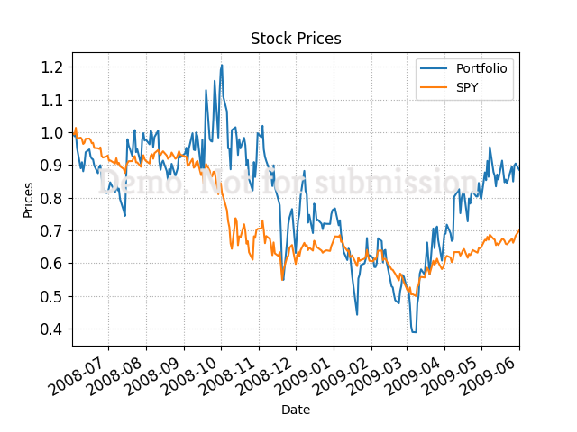
The above is the optimized portfolio. If we instead optimized only for returns, we could expect to see higher overall gains but more volatility. Even though standard deviation is considered, our portfolio only has 4 stocks, so compared to SPY, the S&P 500 index, the volatility is still high.

📖 Assignment 3 - Assess Learners

This assignment goes over decision trees, random forests, and bagging. There are ample resources existing on this topic, so I won't touch on it

Results

We implemented the classifiers from scratch, including determining splits and bagging.

The above diagram shows the effect that leaf size has on bias for training and testing. The leaf size determines the maximum number of samples that can be aggregated into a leaf. So a leaf size of 1 can distinguish every single sample, resulting in a large decision tree, and one that has very low error rates for training.

This low leaf size clearly indicates overfitting, as the testing error is very high. From the figure above, a value of ~10 represents a good balance between bias, variance, and likely execution speeds.

📖 Assignment 4 - Defeat Learners

This assignment involves generating two random datasets.

• Linear regression performs significantly better for inference on one than decision trees
• Decision trees perform significantly better for inference on the other than decision trees

Both learners would be trained and tested on the same data.

Since the deliverable involved analyzing the tradeoffs between the two, I won't touch further on the subject, but there are many resources available which can help you develop a simple method which works.

📖 Assignment 5 - Marketsim

We begin to simulate a market with buying and selling stocks. The methods here and computation for later sections just covers the basics of trades, and if you're unfamiliar with any of it, you can start here.

Results

We are provided a sequence of trades, and a certain amount of cash to start with. We also have all the market data for the time period, and want to calculate the overall portfolio value for a specified date range.

Date,Symbol,Order,Shares
2011-01-10,AAPL,BUY,1500
2011-01-10,AAPL,SELL,1500
2011-01-13,AAPL,SELL,1500
2011-01-13,IBM,BUY,4000
2011-01-26,GOOG,BUY,1000
2011-02-02,XOM,SELL,4000
2011-02-10,XOM,BUY,4000

The above is the example of a portfolio we want to simulate. Each day, we'll need to readjust the portfolio value based on the stock values for the day. Trades involve subtracting the price from our cash and maintaining the stocks in the existing portfolio.

Data Range: 2011-01-05 00:00:00 to 2011-01-20 00:00:00

Sharpe Ratio of Fund: ???*
Sharpe Ratio of $SPX: ???

Cumulative Return of Fund: ???
Cumulative Return of $SPX: ???

Standard Deviation of Fund: ???
Standard Deviation of $SPX: ???

Average Daily Return of Fund: ???
Average Daily Return of $SPX: ???

Final Portfolio Value: ???

* exact numbers witheld

We also want to output certain statistics about each portfolio, like is shown above. It is common to compare one to an index fund as a judge of performance, since you typically want to beat these funds if you are manually trading. That was the belief, at least, until /r/wallstreetbets came along.

📖 Assignment 6 - Indicator Evaluation

Technical Indicators are calculations based on the price, volume, and other metrics of a security. Traders and algorithms can utilize these as heuristics to find patterns and predict the future movement.

A common indicator is the Bollinger Band, which typically plot an upper bound and lower bound equal to two standard deviations, of the 20-day simple moving average for the price. These bounds and timeframe can be adjusted. When the stock price goes over the upper bound, that indicates that it is overbought and may fall, and if it falls underneath the lower bound, that indicates that it is oversold and may rise.

Another indicator is Relative Strength Index (RSI), which is also based on the moving average and is calculated:

$RSI = 100-\frac{100}{1+\frac{Average Gain}{Average Loss}}$

The standard is to use a 14-day moving average, with bounds at 70 and 30 indicating that a stock is overbought and oversold, respectively.

Results

The assignment was to implement and analyze five technical indicators. Two that I chose were the Bollinger Bands and RSI

The figure below shows the Bollinger bands over JPM. Notice the two red 'X'. These are moments when the stock price is well over the threshold, and the indicator is correct in predicting that the stock would fall, and rise.

We can also observe the same stock and timeframe over the RSI indicator. In this case, the boundaries are at 30, and 70. There is an 'X' marked when the price dipped well below the threshold, indicating that the stock is oversold. In addition, the only time JPM went over the upper bound, the stock quickly dropped.

📖 Assignment 7 - Q-Learning Robot

In this assignment, we implement a Q-Learner from scratch to determine the optimal value. There is no application to trading here, and there are many existing resources for basic reinforcement learning, so I won't add to this section.

I also touched on Q-Learning in my Reinforcement Learning course review.

📖 Assignment 8 - Strategy Evaluation

The final assignment is an open-ended project where we use machine learning methods and technical indicators to trade for our portfolios. The three options are:

• Classification-based learner using the random forest implementation
• Reinforcement-based learner using the Q-learning implementation
• Optimization-based by developing an objective function and using the Scipy module

The available actions are buy, sell, or do nothing for one stock. We don't get to control the number of shares or choose from multiple securities, which keeps the implementation and classifiers rather simple.

Results

At the crux of these learners is effective technical indicators. Our first deliverable is actually to create a manual strategy where we set thresholds to trade based on our technical indicators

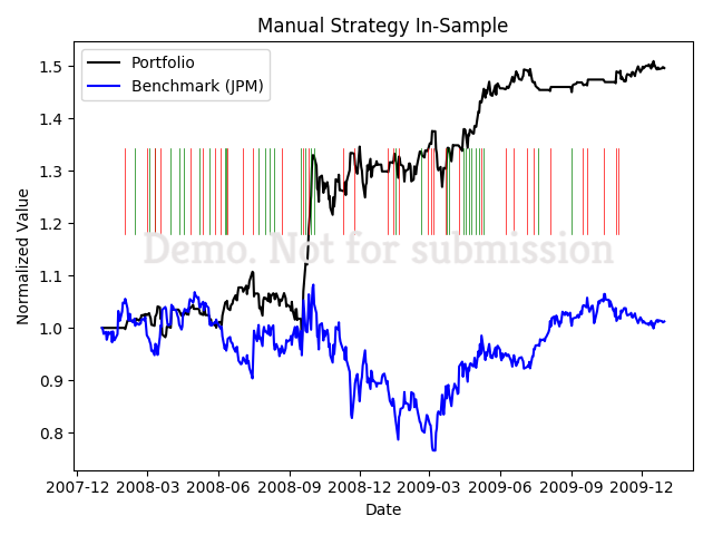
Based on a few technical indicators, I set up basic conditionals to buy or sell. Note that this was optimized to the shown timeframe.

The more effective solution was using a random forest learner to make decisions on when to trade, as is shown below.

The returns generated from the random forest far exceed that of the original stock or my manual strategy. Keep in mind, this represents returns on the training data (overfitting), so the classifier is especially able to take advantage of the volatile periods.

⏩ Next Steps

There is a lack of in depth machine learning strategies, for example, I can't say with much confidence what state-of-the-art approaches entail. There is also not much focus on time-series based methods. However, these are two aspects that are worth looking in to, and the context from this course surrounding finance and ML provides a good starting point.