CS 6644 - Simulation

🔍 Overview

This course provides an introduction to computational, probabilistic, and statistical methods to simulation. Relevant applications are in manufacturing and queueing systems, where simulation can help evaluate the flow through a system and examine demand of parts, which helps inform design choices and resource allocation.

The beginning focuses on the relevant probability and statistics in the domain, and then moves to using the software, ARENA, to graphically generate simulation scenarios and support analysis. There is a also large focus on random number generation and representing processes as distributions.

*I took this course Spring 2020, contents may have changed since then

🏢 Structure

• Homeworks - 10% (of the final grade)
• Two Exams - 60%
• Final - 30%

Homeworks

Homework consisted of multiple choice assignments on Canvas based on the weekly topic, usually involving calculations by hand, and also using Arena, an event simulation software.

Exams

Exams were pretty traditional- also multiple choice and short answer to be completed in a designated time period.

It covered all course content, with a focus on topics that were seen in the homeworks.

📁 Random Variables and Probability Distributions

Note: this course was not project based, and progress was pretty linear. I am not going to go over every single topic. Instead, I will touch on overarching themes to give an idea of what to expect when taking the course.

The inverse transform method enables probability distributions to be be simulated. We'll start with an example which should illustrate some of the statistics touched over this portion of the course.

Let's say we want to simulate a 4-sided die, with equal probability for each side to be landed on. This is a pretty simple task given a Uniform(0, 1) random variable, which is simply a function that maps to a value between 0 to 1 with equal probability for every value in between.

U ~ Unif(0, 1)

• 0 ≤ U < 0.25 ⇒ land on side 0
• 0.25 ≤ U < 0.5 ⇒ land on side 1
• 0.5 ≤ U < 0.75 ⇒ land on side 2
• 0.75 ≤ U < 1.0 ⇒ land on side 3

Pretty simple. Now, let's say this is a weighted die, with sides 1 and 2 having double the chance to land than 0 and 3. The probability for each side is [1/8, 3/8, 3/8, 1/8]. Given the same uniform function, we'll just divide the thresholds of selection accordingly, so:

U ~ Unif(0, 1)

• 0 ≤ U < 0.125 ⇒ land on side 0
• 0.125 ≤ U < 0.5 ⇒ land on side 1
• 0.5 ≤ U < 0.875 ⇒ land on side 2
• 0.875 ≤ U < 1.0 ⇒ land on side 3

Let's visualize this for U = 0.65

If you want to visually simulate this, you just need to see which step U will meet.

Let's look at a graph of the probability mass function (pmf) of this weighted die, which is simply the chance that the a certain side is landed on. We'll also look at the cumulative distribution function (cdf), which is the chance that the side will take a value less than or equal to x, which can be found by taking the integral of the pmf.

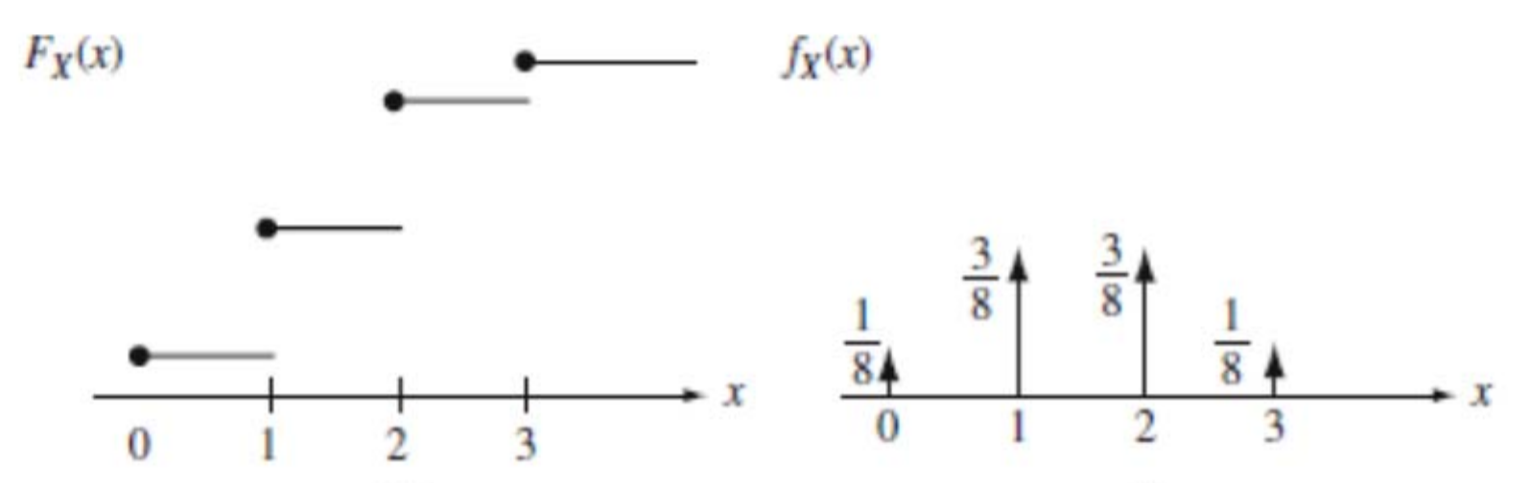
The CDF (left) is the same graph that we used to simulate the weighted die! What we're really doing with that graph is simply taking the value of the inverse of the CDF. If we inverted the X and Y axes, we could simulate the weighted die by calling the inverted function on a uniform variable.

This is the inverse transform method, which allows us to generate samples of a random variable by calling the inverted CDF on a uniform function:

$X = F^{-1}(Unif(0, 1))$

This is really powerful, since we can simulate many random variables with this method.

The figure above shows us sampling an exponential distribution. The probability density function is continuous, formally

$Exp(x)=\lambda e^{-\lambda x}$, and the CDF, pictured above is

$F(x) = 1-e^{-\lambda x}$.

Before, we could visually see how to call the inverse to sample the weighted die. For this method to work, we always need to be able to mathematically determine it, which in this case is:

$F^{-1}(x)=-\frac{1}{\lambda}ln(1-U)$

Practically, 1 - Unif(0, 1) is equivalent to the uniform distribution, so we can simplify the sampling further:

$F^{-1}(x)=-\frac{1}{\lambda}ln(U)$

This module also involved various forms of hand simulations, which are just more hard-coded forms of simulation on simple example, like a stock portfolio and a simple queueing system, both in Excel. In one, the value of pi is simulated

This estimate of pi can be achieved by using two independent Uniform distributions (0, 1), and setting them to be (X, Y) for each point. We then count the proportion of darts that landed in the circle vs outside of the circle, which becomes an estimator for pi, which in this case is 3.176. Given a perfect random number generator, this value will converge to the true value of pi after an infinite number of samples.

📁 Simulation with Arena

Let's simulate a call center!

In this scenario, there are three types of calls: technical support, sales, and order status. Sometimes, the technical support will call you back.

We want to analyze this system to determine wait times and employee effort depending on the number of callers coming in.

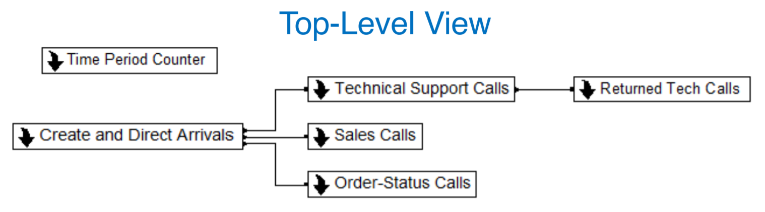
The rate that calls show up depends on the time of the day, so the time period counter keeps track of which 1/2 hour segment we're in.

We'll break down the first module "Create and Direct Arrivals" into more specific components, this time in Arena:

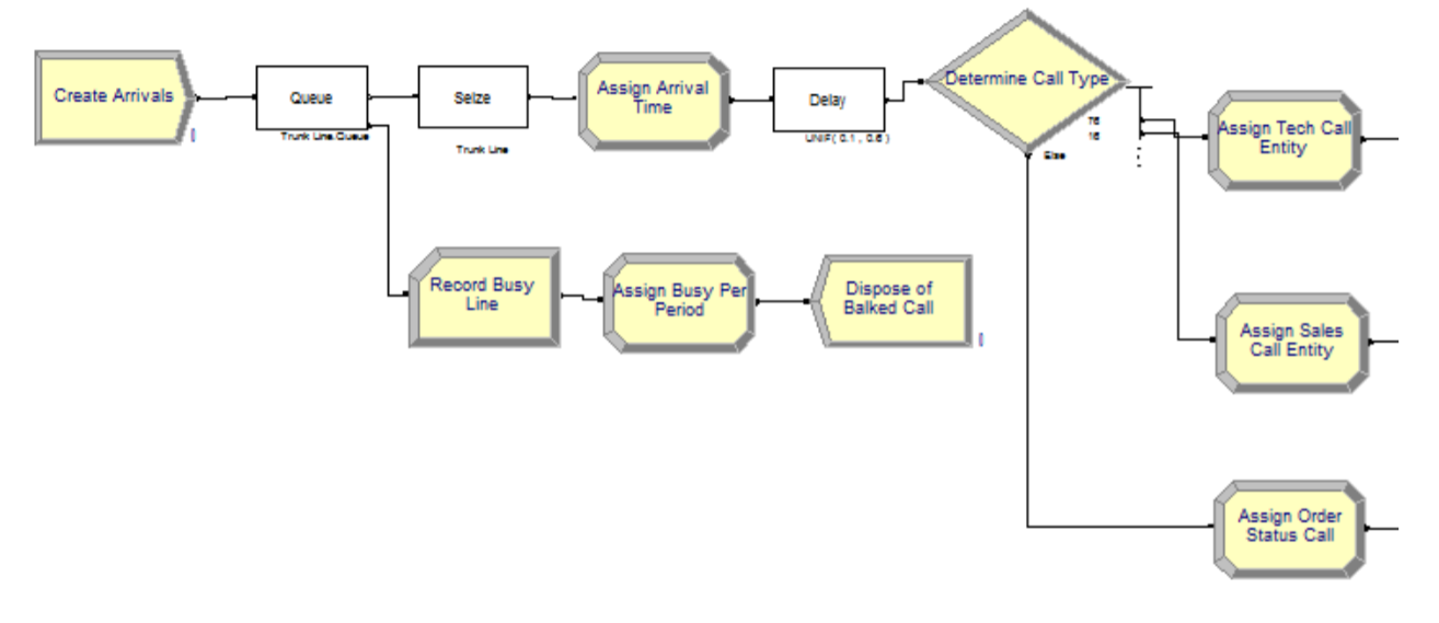
The very first block, "Create Arrivals", simulates the types of callers and frequency they come in at. This can be represented as a Nonhomogeneous Poisson Process. This is actually very simple. The Poisson distribution expresses the probability that a given number of events occur in a specified interval if they occur at a known rate and are independent of each other. For example, from 11:30-12:00, we know the rate is 90 calls, so on average there will be 3 calls per minute. We can use this distribution to calculate the probability for 4, 5, or even 6 calls in any given minute. Nonhomogeneous just means that the rate is not constant and changes over time.

The rest of the blocks do as they are named. Putting the caller in a queue if there are no available agents, and assigning then routing to the appropriate agent after a short delay. Now, let's look at the "Technical Support Calls" module from the high-level diagram.

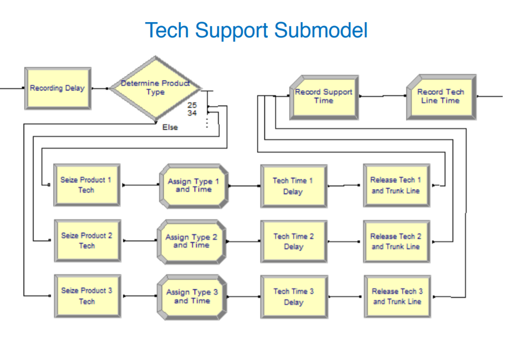
There are three categories of products for the tech support agents, so in Arena, we can add those routes to the module. We can then schedule and label our agents with what they can support:

After running the simulation, the output will contain how long customers were in the queue, how often agents are busy or free, and any other metric you want to observe within the blocks.

There are obviously many more complexities and specifics that I have not mentioned, but in general, the flow-based components in Arena provide flexibility to simulate many scenarios and variables.

Here's an in depth writeup of a simulation using Arena:

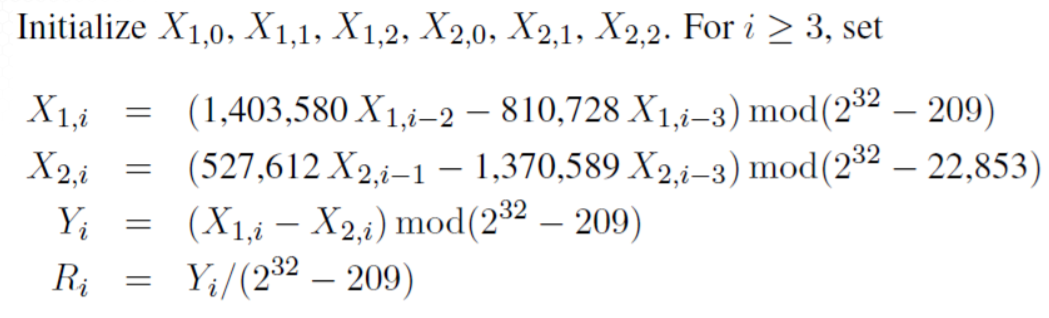
📁 Random Number Generators

In the first section, we used the uniform random variable as a blackbox. This course spends a lot of time covering various methods to generate pseudorandom numbers.

Linear congruential generators, a common technique, are simple to implement and hold good statistical qualities.

$X_i = (aX_{i-1}+c)mod\ \ m$, where $X_0$ is the seed.

$R_i = X_i/m$

R represents the random number, and m determines the cycle length. a, c, and m must be chosen properly to create a reliable RNG. Here's an mini example of an LCG

The RANDU generator was commonly used many decades ago:

$X_i = 65539X_{i-1}mod\ 2^{31}$

However, if you plot $R_{i-2}, R_i, R$ on a 3D graph, you get this:

So while sequentially it may seem fine, there are strong correlations. A perfect RNG would show an equally distributed block if any order of outputs was plotted.

Here's a good generator, with a huge cycle length of $2^{191}$, which practically, has likely never been hit across all random numbers ever computed.

$\chi^2$ Goodness-of-Fit Tests

We can test whether or not our pseudorandom number generator actually generates a uniform distribution by a chi-squared test. There's so much out there about this, so I'll just touch over it briefly. Essentially, you divide your generated numbers into buckets, and compare the difference between the count and the expected count. If this difference is large, we can reject the uniformity of the RNG.

Independence Tests

This isn't enough, as we saw this the RANDU generator. Ordered, evenly spaced numbers within the range would also pass the chi-squared test, so we also want to show that $R_0, R_1, ..., R_n$are independent.

A run test is a simple way to evaluate a RNG, consider the following sequence:

A run occurs when the + or - is repeated multiple times. We don't want too small a value for the number of runs, and we don't want any runs that are too large either.

Random Variate Generation

From the first section, we used the inverse transform method to sample from probability distributions by using the inverse of the CDF. In cases where the CDF cannot be inverted, we can use Acceptance-Rejection

If we want to sample from pdf f(x), but the cdf F(x) cannot be inverted, then we can use t(x) and h(x), pictured below, to sample from f(x)

t(x) and h(x) have the properties:

$t(x) \geq f(x)$ for all x

$h(x) \equiv t(x) / c$

$c \equiv \int_{-\infty}^{\infty}{t_x}$

The constant c makes h(x) have an area of exactly 1

Now, we sample point Y, pictured above, from h(x). And with probability f(y) / t(y), we accept the value and output it as our sample for the distribution.

It's pretty amazing that this works, especially with its simplicity and efficiency. Here is more information and a proof on the theorem.

📁 Input and Output Analysis

Input analysis

We use random variables to adequately approximate the real world. In the call center demo, we utilized the Poisson distribution. This selection is very important- how helpful would the simulation be if we simply had a uniform rate of callers?

For discrete inputs, the following are popular distributions

• Bernoulli - success of an event with probability p
• Binomial(n, p) - # of successes in n Bernouilli(p) trials
• Geometric(p) - chance of this # Bernoulli(p) trials before 1st sucess
• Poisson - # arrivals over time
• Empirical - directly use the measures from a sample

And for continous:

• Uniform - if not much is known about the data, we can start here
• Triangular - if we know the min, max, and most likely values
• Exponential - interarrival times from a Poisson process
• Normal - heights, weights, IQs, etc
• Beta - good for bounded data
• Gamma, Weiball - representative of reliability metrics
• Empirical - directly use the measures from a sample

Given an input data sample and a chosen distribution, we can again use the chi-square test to see if it is an appropriate decision.

Output analysis

There are two types of outputs we typically want to examine, finite horizon (short term) and steady state (long term).

A finite horizon example is rush hour for a transit system. During this short time period, even if you model your simulation perfectly, the random factors will result in varied outputs. Instead of one run, we can replicate the scenario many times, which can help produce an average scenario as well as a 95% confidence interval for the mean.

Steady state analysis can apply to a manufacturing supply chain, which runs for long periods of time without significant change. In this case, while we don't need as many replications, we want to ensure that the initialization parameters are accurate to the real scenario.

⏩ Next Steps

This course provides a good base of understanding for statistical simulation, though it does focus on aspects within the theory more-so than application.

I will be taking the knowledge from this course and try to apply it towards relevant problems. For example, if we want to simulate the operation of a delivery network, can we model customer ordering rate, driver location, to determine what the optimal balance is?

**