CS 6601 - Artificial Intelligence

🔍 Overview

Artificial Intelligence covers relevant and modern approaches to modelling, imaging, and optimization. There is a large focus on implementing algorithms from scratch, and then applying some portions on practical examples. Many of the concepts are at a lower level than you might expect, too, including tasks to optimize runtime. There is probably a higher number of topics in this single course than any other I've taken, though the depth within each varies.

*I took this course Fall 2019, contents may have changed since then

🏢 Structure

• Six assignments - 65% (of the final grade)
• Midterm Exam - 15%
• Final Exam - 20%

Assignments

Six assignments are assigned and due every two weeks, and consist of a problem set where you implement functions to pass an autograder, as well as output additional images for a report.

1. Swap Isolation - Minimax decision making to beat an agent in a board game.
2. Search - Working up from UCS to efficient tri-directional search
3. Bayes Nets - Implementing Bayesian sampling methods
4. Decision Trees and Forests - Implementing the classifier and leaf splits from scratch
5. Expectation Maximization - Clustering methods applied to image segmentation
6. Hidden Markov Models - Demonstration of time series data classification

Exams

These are actually uniquely interesting (and long!), covering topics from assignments, but also those from lectures. You typically solve smaller puzzles by hand using methods to demonstrate knowledge. It is open book + open internet and you have the week to submit.

This includes topics like optimization algorithms, constraint satisfaction, probability and Bayes' Theorem (more in depth), machine learning implementations (neural net, SVM, regularization), time series classification, and Markov decision processes.

Yes, this course is time consuming 🙂

📖 Assignment 1 - Swap Isolation

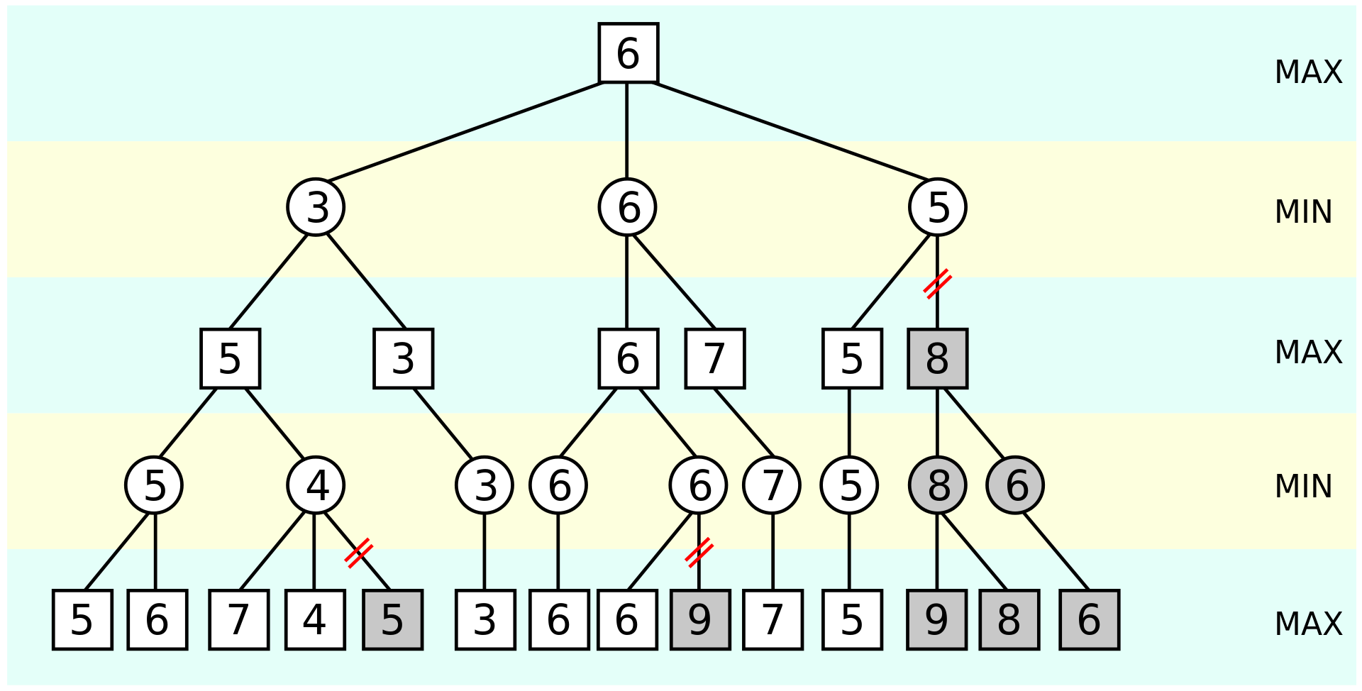
Minimax is a decision-based strategy to minimize the worst-case loss.

The tree above represents a two-player game where each player alternates taking turns. The value at each node is our evaluation for the board, and each connection is an action we can choose to take. The first level, 0 (max), is our turn, so we want to maximize the next situation. then, it is the other player's turn, so we assume they try to minimize our value.

This continues for as deep as we can go, given the computational resources we have.

Alpha-Beta Pruning is an optimization which decreases the number of nodes that need to be valuated, while still guaranteeing the same minimax solution.

Whenever the maximum score that the minimizing player (the "beta" player) is assured of becomes less than the minimum score that the maximizing player (the "alpha" player) is assured of (beta < alpha), the maximizing player can prune further descendants of this node, as they will never be reached in the actual play

Results

We apply minimax and alpha-beta pruning to the game, "Swap Isolation", to beat various players, of increasing difficulty.

This game takes place on a 7x7 grid, with two players that can move with chess queen-like moves. When they move, the space they previously occupied is blocked, so you cannot move through it or move to it again. There is a special move, the swap, where you can swap spaces with the other piece, but this time you can move through the blocked spaces. A swap then has a cooldown of 1 move.

The game ends when a player can no longer make any moves, and they lose.

We apply minimax to beat the other player, including competing agents across other students.

The game tree quickly expands after a few moves, and we get 1 second to make a decision, so to receive full marks, you need to be clever with your implementation.

📖 Assignment 2 - Search

A quick recap on search. Uniform cost search (UCS) expands nodes based on the lowest cost path. We are guaranteed to find the optimal path from start to goal.

A* search achieves better performance by using heuristics. If we use an admissible heuristic, we are guaranteed to find an optimal solution. An admissible heuristic is one that never overestimates the cost to the goal.

We can further reduce the number of expanded nodes while guaranteeing an optimal solution by using bi-directional search. With this technique, we expand from both the start and the goal, and continue until they meet in the middle. Let's compare these with a visualization.

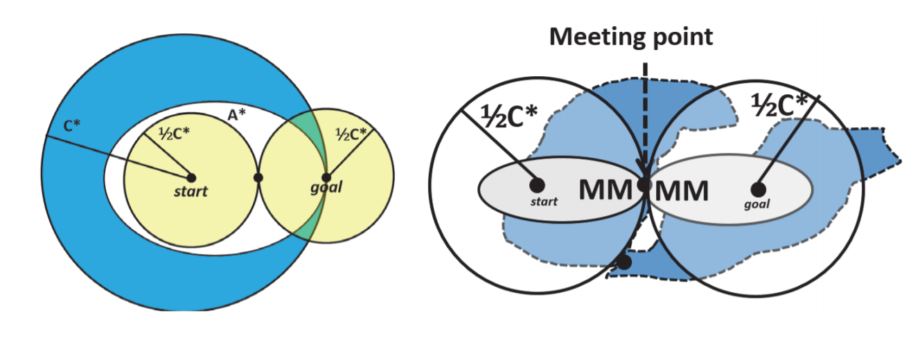
On the left, the large blue circle represents the expansion area of UCS from start, the smaller yellow circles are if we used bi-direction USC. The overall area is significantly reduced. The white oval is A*, which did not need to expand as far left due to its heuristic.

On the right, an improved bi-directional search utilizing heuristics is used, further reducing the search space to find an optimal path.

You need to be careful about the stopping condition though, since it does not necessarily occur on the first node that the two searches meet at. Instead, it is at the point where the the cost of the connecting path is less than the sum of the cost for the two nodes on the frontier. With this condition, we can guarantee that any more connected paths will be more expensive than the existing one.

We can go even further with tri-directional search. In this case, if our goal is to return any valid path going through all three, the heuristic from start A to goals B, C, for a new node becomes the minimum estimate between B and C.

Results

For this assignment, we implement all of these searches and apply them to the infamous Romania graph, as well as an actual map of Atlanta!

📖 Assignment 3 - Bayes Nets

For this course, we use Bayes Theorem for inference on Bayes Nets and distribution sampling.

Bayes Theorem: $P(A|B)=\frac{P(B|A)P(A)}{P(B)}$

In a Bayes Net, events are represented as nodes, and connections show dependence

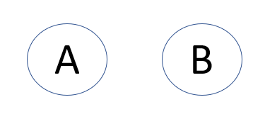
Here, A and B are independent events

$P(AB)=P(A)P(B)$ and $P(A|B)=P(A)$

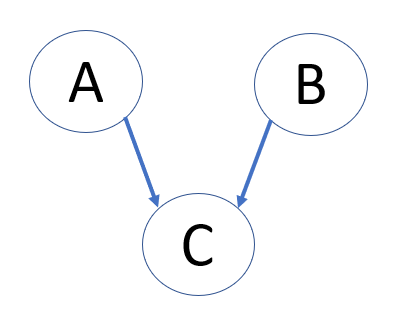
Let's introduce event C, which influences both events A and B

Now, A and B are conditionally independent. Knowing the outcome of event A actually influences our estimate of event B, so $P(A|B)\ \neq P(A)$. You can derive this using total probability and Bayes Rule. As an intuitive explanation, let's say A and B are two independent but accurate cancer diagnosis tests. If we know don't know if a patient has cancer (event C), knowing the result to test A informs our estimate of cancer, which in turn informs our estimate to the test B diagnosis result.

This represents conditional dependence. A and B are independent events that both influence C. Here, C is the confounding cause, and in the absence of information about event C, A and B are still independent. So, $P(A|B) = P(A)$ but $P(A|B, C) \neq P(A|C)$. Here's the best example of this.

Now, we can take this knowledge and apply it to any Bayes net configuration!

Results

This assignment involves properly modeling a Bayes Net as an input to pgmpy, a Python library that assists in Bayesian inference. It uses variable elimination to solve for the posterior.

We also implement Gibbs Sampling to estimate for a more complicated network.

📖 Assignment 4 - Decision Trees and Forests

Decision trees are often the best performing learner for tabular data. That is, after some clever optimizations on the vanilla implementation. See: XGBoost and LightGBM

Because of the ample resources, I won't touch much on decision trees and forests, as this assignment simply involved their implementation.

📖 Assignment 5 - Expectation Maximization

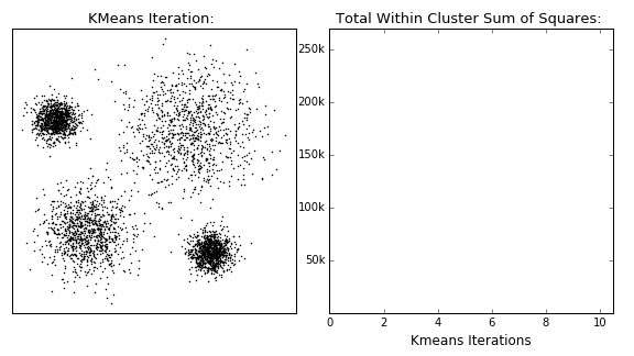
K-Means Clustering is an unsupervised (does not require labels) technique which groups data points into 'k' clusters, each with a computed center, where point belongs to the cluster with the nearest center. Its aim is to group similar data points together and identify underlying patterns.

The algorithm is guaranteed to converge, but there also exists local optima, so restarting with changed initial locations may be necessary to find the optimal clustering.

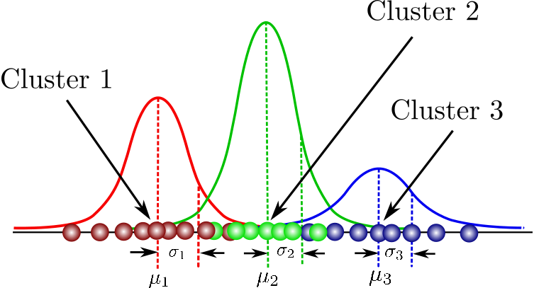
Let's address some problems of k-means: what if some of the clusters are overlapping? Or if a cluster has a non-circular shape? Gaussian Mixture Models (GMM) ****cluster as Gaussians, and assign a probability distribution for the center, as well as having a covariance distribution which describes their shape. This allows us to assign data to a cluster by some probability.

A GMM consists of different Gaussian components, and the joint distribution is described by the weighted average of the individual components

Expectation-Maximization (EM) is the iterative algorithm which optimizes the parameters of the GMM. For more information on GMMs and EM, refer to this excellent video!

Results

We implement a vectorized version of k-means clustering and apply it to images. The gif below shows the clusters from k = 2 → 6 over the original image, on the left. In the end, the grey, yellow, two shades of blue, and two shades of red are found to be the average colors with the least error across all pixels.

We also implement expectation maximization to utilize GMMS for this same problem, which results in a similar output image.

This same technique can be applied to 3d images, as shown below. Pretty cool!

Objects were still segmented by color, but additional coloring replaced the original shade to provide more contrast.

📖 Assignment 6 - Hidden Markov Models

A Markov chain is a sequence of events with transitions based on certain probabilities. The probability of the next even occurring only depends on the current state. A Hidden Markov Model (HMM) is a Markov chain with unobservable states, X, as well as observable states Y, which depend on X. The goal is to estimate state X based on observed outcomes Y.

The above is a Hidden Markov Model of the weather guessing game. In this situation, Alice walks, shops, or cleans, solely based on the weather with the shown probabilities. Unfortunately her friend Bob is stuck in a basement and cannot directly observe the weather, but Alice tells Bob the activity she did each day. Bob knows the general weather behavior, and what Alice likes to do (the events and transition probabilities are known), so she tries to guess the weather based on Bob's activities.

The Viterbi algorithm is a method for finding the most likely sequence of hidden states.

Results

We implement various methods to estimate the word from ASL videos based on the hand position sequences.

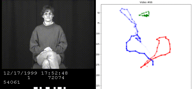
Our model takes the sequence of inputs X and Y from a single hand and guesses the original word. This is modeled by three hidden states for every single word, representing the start, middle, and end of the sequence.

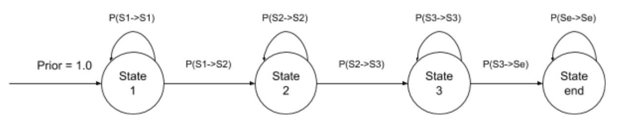
We are given training data, which consists of the original word and its sequence. Given this information, we can model each state for each word by their sequence statistics and apply this model to estimate the base word for sequences we have not seen.

✏️ Exams + Other Topics

I believe it's worth briefly mentioning course topics that were not on the homework assignments but were still covered.

Genetic algorithms are a global optimization technique, best known as a method to solve NP-Hard problems like the travelling salesman problem. An interesting application, for which we had to solve a mini-version of, is multiprocessor scheduling. When you have many tasks with a complicated dependence, solving for the ideal configuration is an NP-Hard problem.

Given certain constraints, you can apply mutations and crossovers to optimize for the schedule

Constraint Satisfaction Problems have a world in which a set of variables can be assigned to a value, as well as certain constraints on those values. Map coloring is a popular example of this, where you need to assign a certain color to each country, but no adjacent areas can have the same color.

This also applies to many graph-based puzzles like Sudoku, and these are typically solved using a search variation. This search is often optimized based on domain-specific heuristics, such as the Minimum Remaining Value heuristic, which chooses the variable with the least possible values given the current configuration.

This article provides a cool visualization on the backtracking search tree for sudoku.

Dynamic Time Warping is a time-series classification technique which measures similarity between two sequences that can vary in speed. Naively, it can be implemented by dynamic programming as shown below.

⏩ Next Steps

I certainly feel more confident with the overall themes, strategies, and even the math. It was beneficial to implement some topics which are not as popular, such as GMMs and AB pruning, as it widens our base compared to seeing similar topics over and over. You are definitely equipped to start understanding research papers within many of these topics.