CS 7642 - Reinforcement Learning

🔍 Overview

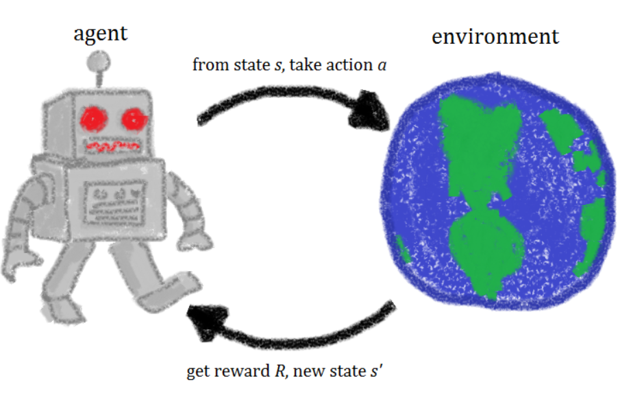
In reinforcement learning, an agent learns to achieve a goal in an uncertain, potentially complex, environment. It has applications in manufacturing, control systems, robotics, and famously, gaming (Go, Starcraft, DotA 2). The theory behind reinforcement learning has been long researched, and it has seen recent success largely due to the massive increase in computational speed and datasets.

This course provides an introduction to reinforcement learning, from theory to practice. It maintains a focus of reading and understand academic papers, while also allowing exploration of modern approaches and frameworks. This involves writing some algorithms from scratch, and a bit of utilizing existing implementations.

*I took this course Spring 2019, contents may have changed since then

🏢 Structure

• Six assignments - 30%
• Three projects - 45%
• Final exam - 25%

Assignments

Submissions were like solving test cases, where we solve a specific input and enter in the output, which a server verifies, and that's our grade. Much of it involves writing methods from scratch, with many possible approaches for each. Occasionally an external library is required, like OpenAI Gym.

1. Optimal State-Value Function - Finding the optimal policy and actions from a game with an N-sided Die
2. TD-Lambda - Temporal Difference algorithms and k-step estimators over a Markov Decision Process (MDP)
3. Defeat Policy Iteration - Designing MDPs with architectures that directly contrast their solvers
4. Q-Learning - Implementing Q-Learning to solve discrete MDPs
5. Bar Brawl - Applying KWIK (Knows-What-It-Knows) Learning, a self-aware learning framework, for outcome prediction
6. Rock Paper Scissors - Game Theory, Nash Equilibrium, and Linear Programming over rock paper scissors variants

Projects

For each of these projects, you submit a report which goes over your implementation, and closeness of results to what is expected. Proper analysis tends to be more important than the actual result, for example, I was not able to replicate a figure well for the last project, but still received a decent grade.

1. "Desperately Seeking Sutton" - Implementing and replicating results from Sutton's TD-Lambda paper, Learning to Predict by Methods of Temporal Differences
2. Lunar Lander - Train an agent to successfully land a 2D rocket, the lunar lander problem on OpenAI Gym
3. Correlated-Q - Implementing and replicating results from Greenwald and Hall's paper, Correlated-Q Learning

Final Exam

A difficult exam that covers any detail over the whole semesters' lectures, assignments, and academic paper readings. The mean was a 50, and the high was a 74 🙂 Final grades are scaled though, don't worry!

📖 Assignment 1 - Optimal State-Value Function

A Markov Decision Process (MDP) consists of a set of states, actions, transition functions, and rewards. I'll describe each according to the figure below, which is an MDP

• States - S0, S1, S2
• Actions - The set of actions available for each state. In this MDP, each state can take a separate action a0 or a1
• Transition Functions - The probability for an action to result in transition from one state to the next. For S0, action a0 has 50% chance to go to S2, and 50% chance to return to S0
• Rewards - The reward for transitioning from one state to another taking a specific action. There are two rewards, +5, -1, present in this MDP.

The Bellman Equation can be used to find an optimal policy, which specifies the best action for any given state.

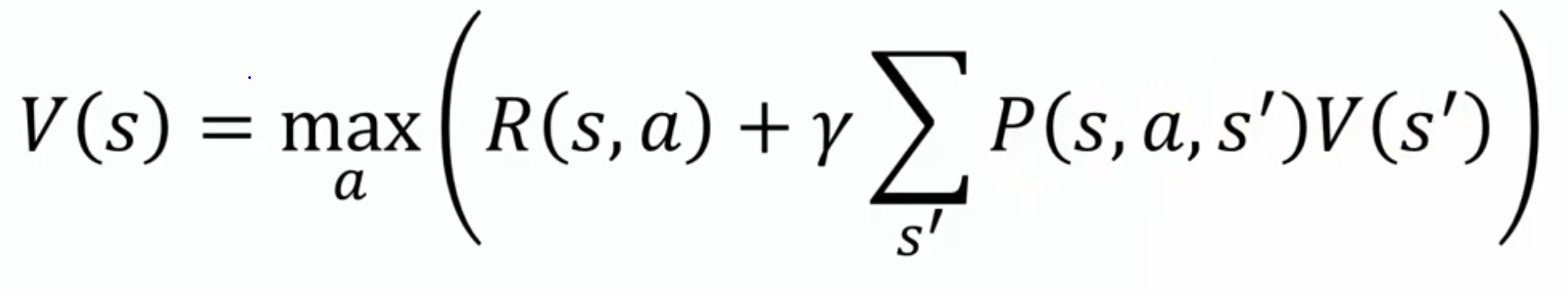
V(s) describes the value at state s. This value is equal to the action which maximizes the immediate reward, R(s, a), as well as the discounted future rewards. Parameter gamma is a value between 0 to 1, which defines how much to discount a reward down the line. Future rewards, take the weighted value of the next states after taking action a, proportional to the probability that they occur.

Results

The game DieN is played as follows:

• You are given an equally weighted die with N sides

• A bit mask vector which will make you lose if you roll them

  • For a die with 3 sides, and vector [0, 1, 0], rolling a 2 makes you lose, but 1 and 3 are safe!

• Any time, you can roll or quit

  • If you roll and hit a safe side, you get that many dollars. With the same die as above, each time you roll a 1, you get $1, each time you roll a 3, you get$3.
  • If you roll and hit a losing side, you lose all your money and the game ends. So if you rolled a 3, then a 2, you gain $3, but lose it all.

For the DieN problem, N = 6, isBadSide = [1,1,1,0,0,0], the expected value for optimal play is 2.5833. In this case, rolling sides 1 → 3 result in losing the game, and 4 → 6 result in gaining that side in dollars.

This problem can be represented and solved as an MDP using value iteration.

How would you represent states, and wat would the transition probability be between states for actions "roll" and "don't roll"?

What would the discount factor be?

📖 Assignment 2 - TD (Lambda)

"Suppose you wish to predict the weather for Saturday, and you have some model that predicts Saturday's weather, given the weather of each day in the week. In the standard case, you would wait until Saturday and then adjust all your models. However, when it is, for example, Friday, you should have a pretty good idea of what the weather would be on Saturday – and thus be able to change, say, Saturday's model before Saturday arrives" -Sutton

Temporal difference learning is a strategy which samples from the environment and performs updates to past states based on the current environment.

In the example below, the first action is taken at the top, and the terminal action at the bottom, so each previous state is updated according to lambda.

David Silver, of DeepMind, has a great video on this topic. The rest of his lectures on reinforcement learning are also high quality, they were helpful for me to gain intuition for many concepts in this course.

Results

Given the following MDP, we want to find a value lambda which produces estimates equal to TD(1).

probToState = 0.81
valueEstimates = [0.0, 4.0, 25.7, 0.0, 20.1, 12.2, 0.0]
rewards = [7.9, -5.1, 2.5, -7.2, 9.0, 0.0, 1.6] # 

Output: 0.622632630990836

In the above case, if we discount the updates with lambda = 0.622, the value estimates for each state equal TD(1). The arrays represent the value estimates and rewards for the six components. probToState is the chance for state 0 to move in the specified direction.

💻 Project 1 - Desperately Seeking Sutton

This project involved recreating figures from Sutton's paper, Learning to Predict by the Methods of Temporal Difference. This involves understanding the paper in depth, and then trying to implement the experiments.

Sutton’s TD algorithms are analyzed with a simple system that simulates bounded random-walks. A bounded random walk is a sequence generated by moving in a random direction until a boundary is reached.

This covers the same TD(Lambda) topic as HW2.

The bounded walk is pictured, and the true probabilities of right-side completion (goal G, outcome 1) are 1/6, 2/6, 3/6, 4/6, and 5/6, for states B, C, D, E, and F, respectively.

Results

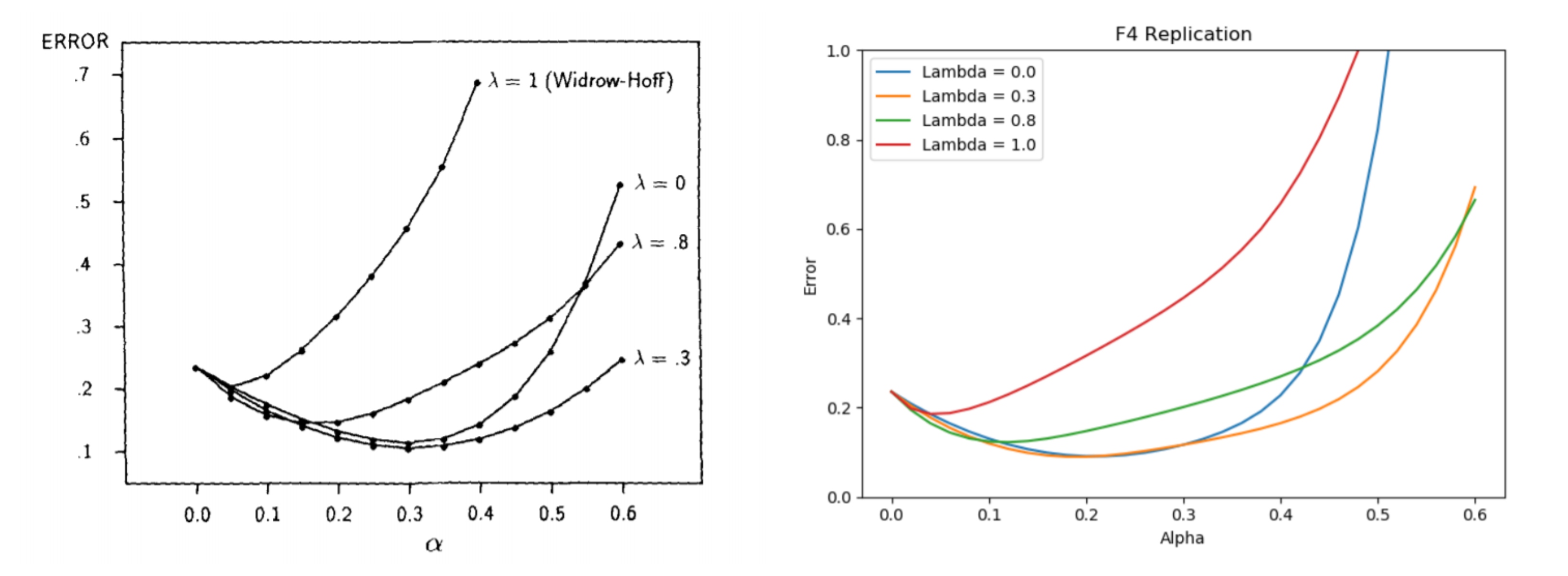
Sutton's experiments involve taking different values of lambda and alpha (learning rate) and averaging the error across many experiments which quickly terminate after a few sequences. In general, you find that TD learning matches the actual probabilities at a faster rate when lambda is selected well.

Below is a comparison between the figure we were to replicate, which has similarities but clear differences as well. Further analysis about why there are differences was a requirement for the report.

📖 Assignment 3 - Defeat Policy Iteration

Value iteration and Policy iteration are common techniques to solve MDPs. They converge to the same solution and are both similar but have distinct differences, which results in varying runtimes for different MDPs.

Value iteration takes the Bellman equation and turns it into an update rule. Each state is visited, and the best action is chosen, and rewards are propagated depending on the discount factor. This repeats itself until the change in policy is smaller than some threshold.

Policy Iteration

For policy iteration, all states are evaluated, and then there is an update. This results in convergence over fewer iterations, but not necessarily fewer overall operations.

Results

The task of this assignment was to design and MDP that takes at least 15 iterations to converge with policy iteration, with some constraints on how our MDP could be designed.

As inspiration, the MDP below was discussed in the course, and it takes exponential time to converge. Although all states and actions are evaluated each iteration, converging to the optimal solution with policy iteration takes longer as the values propagate slower than with other designs.

📖 Assignment 4 - Q-Learning

Q-Learning is the base concept of many methods which have been shown to solve complex tasks like learning to play video games, control systems, and board games. It is a model free algorithm that seeks to find the best action to take given the current state, and upon convergence, learns a policy that maximizes the total reward

It is built on the concept of exploration vs exploitation, where the agent will take the best predicted action so far, or take a random action with epsilon chance.

This method maintains a table of Q-Values, which assigns every state and action with a expected reward. This is similar to the values from V(s) of value iteration and policy iteration, but a key difference is that the agent does not need to know the MDP model (hence model free) to directly update based on known probabilities of taking actions.

Results

We apply Q-Learning to solve the Taxi problem, a discrete MDP. There are 4 locations (labeled by different letters) and your job is to pick up the passenger at one location and drop him off in another. You receive +20 points for a successful dropoff, and lose 1 point for every timestep it takes. There is also a 10 point penalty for illegal pick-up and drop-off actions

OpenAI Gym is an open source project, and the source code for this problem can be viewed here. It is a simple API which defines the environment, takes actions, then assigns state and reward.

💻 Project 2 - Lunar Lander

Lunar Lander is another OpenAI environment in which we want to land a rocket safely into a target location in a 2D environment. The rocket has four actions- to use the left booster, right booster, bottom booster, or do nothing. Below we see two animations, one agent taking random actions, and the other, a trained agent, landing safely!

To solve this problem, we'll need to look towards more complex models than those that have been visited earlier in the course. Three common approaches are Deep Q-Learning, Actor-Critic, and the Cross Entropy Method.

Deep Q-Learning extends the Q-Table to be a deep neural network to be the input, often a convolutional neural network, with the action selection being similar to classification outputs in other machine learning problems.

Actor-Critic takes two networks, the actor- which determines the action when a state is given, and critic- which evaluates the value of the state

CEM is similar to the genetic algorithm, which runs the agent through many sessions, selects the best performing rounds, and trains on those inputs and outputs.

Results

Our requirements were not just to successfully land our agent in the goal once, but to Have the average reward reach at least 200 across 100 episodes. Below you can see some of my results, which include the learning curve and distribution of episode rewards across my successful submission.

Part of the overall Lunar Lander challenge (not this project) is to be able to efficiently find a good performance- an agent that can learn a passing solution with few episodes. Mine was very ineffective in that regard, as it took many episodes to reach the average reward requirement.

Poor learning w.r.t number of samples used, especially compared to humans, is a huge problem and criticism of reinforcement learning in general. Some say agents are simply overfitting to data points and cannot generalize.

📖 Assignment 5 - Bar Brawl

A KWIK (Knows What It Knows) is a framework where a learner can respond with "I DONT KNOW" as an output. This is apt for efficient active learning, as the agent can select the data it wants to learn from. An intelligent learner can be more sample efficient than one that randomly chooses actions.

We want to solve Bar Brawl. For this problem, a bar is frequented by n patrons. One is an instigator, and when he shows up, there is a fight, unless another patron, the peacemaker, is present at the bar.

On a given evening, a subset of patrons is present at the bar, and our goal is to predict whether or not a fight will break out without knowing the identity of the instigator or peacemaker.

Results

In the example problem, we are given a tuple of whether or not the instigator or peacemaker are present, and whether or not the fight occurred. If we confidently answer yes or no to a fight occurring, we move on to the next round, otherwise we say I dont know, and are given the result. Let's walk through this

(true, true) - we don't know who is the instigator, but both are present, so we can confidently say there is no fight

(true, false) - since we still don't know who is who, we must say I dont know. After this, we are told that a fight did occur

(false, true) - since we know that a fight occurred, we are confident that patron at index [0] is the instigator, so now we know a fight did not occur!

(true, true) - both are present again, so a fight does not occur

(true, false) - now that we know the instigator is the first, we know a fight did occur

The problem becomes more complicated when there are more patrons, and for this assignment, we are limited in how often we can say "I DONT KNOW".

📖 Assignment 6 - Rock Paper Scissors

Nash equilibrium occurs when no player wants to deviate from their chosen outcome after considering the opponent's choice, and is the optimal outcome.

The popular thought problem which illustrates this well is the prisoner's dilemma, where the Nash equilibrium is for both players to defect against the other, despite cooperation resulting in a better reward.

For typical Rock-Paper-Schissor, the optimal action is actually a mixed strategy, where you choose between the three with equal probability.

However, let's consider a scenario where not all combinations result in equal outcomes, like the one below. The optimal strategy becomes one that is not an equal distribution.

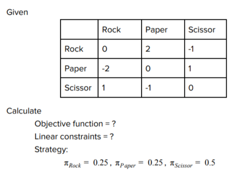
Linear programming is an efficient method to solve for the Nash equilibrium, which we can use existing libraries to solve for. In linear programming, we seek to maximize an outcome given an objective function and a set of constraints

Results

Don't worry, we don't need to implement a LP solver. Rather, we need to successfully define the constraints and matrices as an input for the rock paper scissors variants. We can utilize the Python library cvxopt for this. Unfortunately there's not much else to show for this problem, as any next step would be part of the solution.

💻 Project 3 - Correlated-Q

Multi-agent learning involves an environment with multiple agents which can interact with each other. This is a very active research area with huge potential for defining how robotics and complex systems will behave in the future.

For this project, we consider soccer, a zero-sum game which does not have a deterministic equilibria.

"The soccer field is a grid. The circle represents the ball. There are two players, whose possible actions are N, S, E, W, and stick. The players’ actions are executed in random order. If this sequence of actions causes the players to collide, then only the first moves. But if the player with the ball moves second, then the ball changes possession. If the player with the ball moves into a goal, then he scores +100 if it is in fact his own goal and the other player scores −100, or he scores −100 if it is the other player’s goal and the other player scores +100. In either case, the game ends."

With the illustration, we can see how a deterministic policy cannot be optimal. If "B" always moves right, the A can indefinitely block. If "B" always moves down, the A can move down too. However, if "B" chooses their action over a probability distribution, then they will sometimes be able to reach the goal.

Defining a value function in multi-agent learning is more subjective, as there are variants in how you want to prioritize outcomes.

Friend-Q seeks to maximize any and all reward, where any player's reward is equivalent;

Foe-Q, in contrast, treats the other agent as an adversary and seeks to maximize the worst-case scenario that the other agent can put them in. This is the same as minimax.

Correlated equilibrium, for Correlated-Q, is a probability distribution over the joint action space, in which agents optimize with respect to one another’s probabilities, conditioned on their own.

Results

Similarly to project 1, our task is to recreate figures in Greenwald's paper, Correlated-Q. This involves creating a replica of the soccer environment and then successfully defining the constraints and objectives for the various forms of Q-Learners.

The figures illustrate the Q-value differences from the previous iterations.

Q-Learning differences. Since Q-learning aims to find a deterministic policy, it never converges.

Here, both Correlated-Q learners converge in a somewhat similar pattern.

Although my figures were closely matched, my Correlated-Q actually converged on a different policy than that of Greenwald's, which resulted in a reduction on my project.

✏️ Final Exam

The final exam involved topics beyond those from the assignments, so I will briefly mention some.

POMDP (Partially Observable MDPs) do not have the entire state space visible. Video games often fall into this category, whereas board games have the full state viewable by all players.

Inverse Reinforcement Learning aims to extract a reward function from an environment given observed, optimal behavior

Policy Shaping utilizes human feedback as direct labels on a policy to interactively train RL systems.

...and many more!

⏩ Next Steps

This course increases confidence in reading academic papers and understanding notation in reinforcement learning. Paired with the high-level tasks, you definitely become equipped to implement more tasks in OpenAI Gym, and other benchmarks. Also, you start to understand the jargon of AlphaGo Zero, AlphaStar, and other newsworthy breakthroughs!

I'm interested in learning more about reinforcement learning applied to robotics control systems. Continuing off of the lunar lander project- how realistic might this strategy be for landing a SpaceX rocket? Can Boston Dynamics begin to teach their robots to walk through a combination of physics simulation and real experimentation?